The software PASAD-tools provides a Digital Micrograph® plugin with graphical interface for automatic and fast determination of quantitative data from selected area electron diffraction (SAD) patterns. Version 2.0 provides a new user interface (more flexible and easier to use), new functionality (e.g. the possibility to possible to calculate the radial distribution function) and a lot of bug-fixes. The software can be used free of charge under the condition a reference is made to the following publication (or a newer PASAD publication): http://dx.doi.org/10.1016/j.scriptamat.2010.04.019.
This is a short documentation for the functions provided plugin. You can also consult the PDF included in the download. Feel free to contact me any kind of questions, bug reports or feature requests.
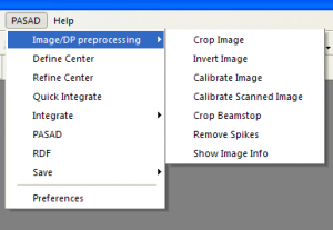
Graphical interface
Some tips on the use of the software:
Click on a function while holding shift to get help.
Always bring the image you want to work on to the front
Installing the software
For an improved speed the PASAD-tools were partly written as Dynamic Link Library.
To install the plugin both the “PASAD-tools.dll” and the “PASAD-tools.gt1” have to be copied to the plugin directory. Make sure you use the correct version, depending whether you use Gatan Microscopy Suite® 2 or an older version of DigitalMicrograph®.
Image preprocessing
Crop Image
Bring the desired image to the front and select the region to be cropped using the rectangular region of interest (ROI) tool. Then click on “Crop Image”.
Invert Image
Bring the image to the front and click on “Invert Image”. This is only necessary for scanned films.
Calibrate Image
Opens a dialog allowing to calibrate the image/profile from a given distance. (If a profile was acquired from a SAD the calibration will automatically applied to both.)
Alternatives for images: Draw a single point ROI having a certain distance to the center (has to be defined first) OR draw a line ROI with a given distance. Then use the function.
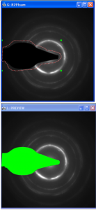
The entire beamstop is selected using the ROI tools (top) and then refined (bottom)
Alternatives for profiles: Draw a tight ROI at a known position OR draw a ROI with a known width. Then use the function
Calibrate Scanned Film
Allows to calibrate a scanned image/diffraction pattern from the resolution[dpi] and the magnification/camera length.
Crop Beamstop
The procedure works in 2 steps: Use ROI tools to cover the entire beamstop (see figure to right). To mark multiple ROIs hold shift. Then use thisfunction. If no ROIS are found in the image, an assisted procedure is used that allows to mark the beamstop using 1 or 2 rectangles. The second step will allow to crop everything or refine the region to be cropped by clicking on the brightest point in the beamstop (this is usually at the edge near the central beam). In the figure on the right the result after refining is shown.
Once the beamstop is cropped it will be ignored in the integration leading to more accurate profiles.
Remove spikes
This function allows to remove outliers in the front image. Pixels differing more than a threshold from the median of the neighboring pixels are replaced by the median. A warning is given if more than 5% would be removed.
Find Center
Define Center
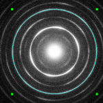
A center indicated by a ring.
This allows to define the center in the front image by clicking on 3 point on a ring or double-clicking on the center.
Alternatively define the center by drawing a point ROI or a circle and then use the function.
Refine Center
After defining the center you can refine the center using downhill-simplex. Keep the ALT-Key pressed if you want elliptical distortion correction. The ellipticity values are stored in the image tag “PASAD” and the center is defined as origin. The values can be changed manually. The center refinement is done using a Downhill-Simplex-algorithm. The most intense ring is chosen, and the center of integration is moved until the peak in the azimuthal integral is maximally sharp, which is the case if the peak height reaches its maximum.
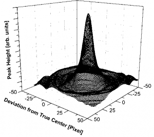
Peak height in dependence of the deviation of the center of integration from the true center,
Integrate
Use azimuthal integral for profile analysis and azimuthal average for RDF analysis.
Quick integrate
This function is used to do an azimuthal integral of the front image with high precision. If there are ellipticity values in the image tag, elliptic corrections are taken into account. The integration limit is the largest circle. The profile will be linked to the SAD.
Other integrate functions
Azimuthal Integral / Azimuthal Average: Azimuthal integral/average allowing to select the maximum radius.
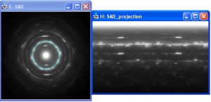
SAD pattern and corresponding azimuthal projection
Azimuthal Projection: Allows to do an azimuthal projection (x-axis=angle, y-axis=radius) of the front image. To get an azimuthal projection with full resolution hold ALT key. The azimuthal projection ignores ellipticity.
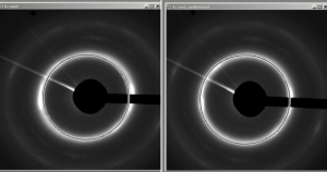
Distorted SAD pattern (left) and undistorted (right)
Elliptic undistort: Allows to undistort a front image with elliptic distortions.
If center refinementincluding elliptic correction was used this values will be used, otherwise the user will be asked to enter ellipticity (a/b) and theta[°] (angle of the larger axis with the x-axis measured counterclockwise).
Peak fitting
Find Peaks
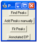
Dialog showing the profile analysis functionality
After the electron diffraction profile was obtained by azimuthal integration, the peaks can be determined automatically using the “Find Peaks” button.(In the new version you can also start directly from a profile.) To get a good result set a ROI to the area of interest (just drag over the region with the left mouse button pressed). Optionally you can also zoom to the desired ROI. (The peakheight threshold in the preferences allow to distinguishing between peaks and noise.)
At the minimum points between the peaks, splinepoints are set for background subtraction. Between peaks with an overlap no splinepoints are set. (This is determined by the peak-overlap threshold in the preferences.) The background determined using the splinepoints is subtracted from the profile.
Each individual peak is fitted using a Voigt peak-fit. The peaks together with the profile and the background are then plotted so that the user can change the parameters if necessary or add and delete any peaks.
Add Peaks manually
Screenshot showing peaks indicated by ROIs and splinepoints indicated by circles.
It is also possible to add and delete peaks or splinepoints manually. After selecting “Add Peaks manually” peaks are indicated by ROIs and splinepointsare indicated by small circles in the profile (see figure to the right). To add a peak click on the desired position using the left mouse-button. Click on a peak using the left mouse-button while holding ALT to delete this peak. To add a splinepoint click on the desired position using the middle mouse-button. Click on a splinepoint using the middle mouse-button while holding ALT to delete this splinepoint. When ready press ESC. For help press “h”. In the new version you can also start without prefinding.
Fit Peaks
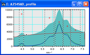
After that, a model including all the peaks is fitted to the background subtracted profile, the splinepoints are then moved according to the value of the fit and a second fit is performed to the corrected profile. The fit results will be displayed.
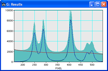
Screenshot showing the raw data (filled), the background (red), the background subtracted data (green) and the fit to the background subtracted data (blue).
Annotated diffraction pattern
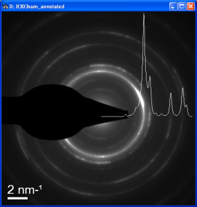
By selecting Annotated DP a SAD pattern with a scalebar and an inserted background subtracted profile is created. (In GMS2+ you can increase the line thickness or change its color using right click-Image display.)
Save results
Save as XLS
This function allows to save the PASAD profile (has to be the front image) as .xls format. You can also save other images or profiles using this function. The function makes use of calibrations and slice names.
Save as DAT
Same as above but the profile is saved as space separated text.
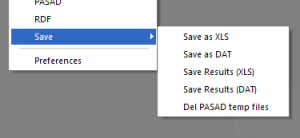
Save result (XLS)
Saves PASAD fit results (peak position, width, intensity and shape factor) in .xls format. Bring the profile to the front first. The information is taken from the hidden peakparameters image.
Save result (DAT)
Same as above but the results are saved as space separated text.
Delete PASAD temp files
Deletes all the hidden PASAD splinepoint and peakparameter images. While you are using PASAD do not mess with the hidden images because they contain all the fit information. But after fitting many profiles you can have lots of hidden images, and they can be removed using this function.
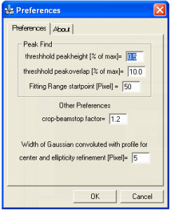
Preferences
This brings up a dialog allowing to change some default parameters for PASAD. Peakheight threshold: Peaks smaller than this height are ignored (the height is given in percent of the profile maximum). Peakoverlap threshold: If peaks have an overlap bigger than this height, no splinepoint is set between these peaks (height given in percent of profile maximum). Fitting range startpoint: If no region is selected the peakfind will start at this pixel. This is done to ignore beamstop artifacts. Crop-beamstop factor: The intensity selected during refinement is multiplied with this factor before thresholding. Width of Gaussian convoluted with profile for center and ellipticity refinement: This can help to prevent the center value running into one of the two focal points for very elliptic patterns.
PASAD-RDF
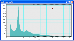
Set a ROI at the end of the profile before fitting background
For a RDF analysis do the following steps:
Crop beamstop; Find and refine center; Calculate the azimuthal average (use the maximum range)
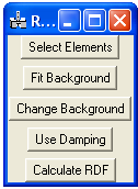
Then go to the RDF menu:
Select elements: This is necessary to calculate the scattering function, the Kirkland scattering function is used (for more information refer to the book “Advanced Computing in Electron Microscopy”).
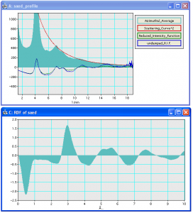
Top: window showing azimuthal average, scattering curve squared and reduced intensity function Bottom: reduced density function
Fit background to curve (first set a ROI to the range that should be used for fitting, see figure to the right).
You can change the background if you do not like the results. (In GMS2.0 OK and Cancel will not close the dialog as there is a bug, just close it manually after clicking.)
A window showing the azimuthal average, scattering curve squared and the reduced intensity function will be shown (see figure to the right).
To get rid of the noisier part in the higher values use damping. A Gaussian damping function is used and the dialog allows you to set the value where the curve is reduced to 1/e (i.e. higher values mean less damping). The damped and undamped function will be displayed
Once the reduced intensity function looks fine, use Calculate RDF. Select a ROI to exclude some area. By default the reduced density function G(r) will be calculated. To calculate the radial distribution function, hold the ALT key.
To save the profile or RDF use Save as XLS/Save as DAT.
Acknowledgment
This script would not have been possible without helpfiles and scripts from many other people, mainly Dave Mitchell and Bernhard Schaffer. The scripting homepage http://dmscripting.com (by D. Mitchell), the script database http://portal.tugraz.at/portal/page/portal/felmi/DM-Script and the DMSUG mailing list are essential for every scripter. Furthermore I would like to thank Martin Peterlechner for the help with scattering factor and RDF calculations.
